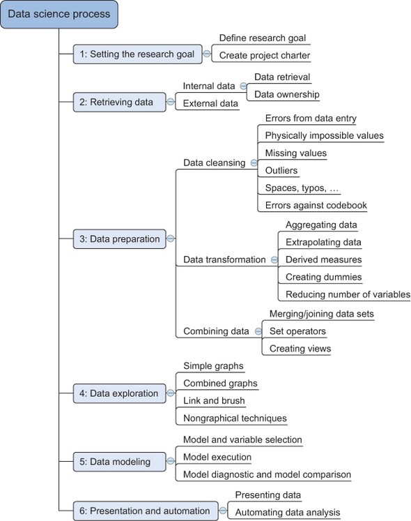
The Data Science process consists of various steps. The image below represents six steps from Setting the research goal to Presentation and automation. As a beginner in the Data Science field, I am doing some projects on Data cleaning and analysis.

In this story, I will share What is Factor analysis? and then a project I have done on Hotel satisfaction scores.

Introduction to Data Science by Manning

What is Factor analysis??

Factor analysis is a dimensionality reduction technique (reducing the number of features), which could be exploratory or confirmatory. The main objective of Factor analysis is to reduce the number of variables in the study and replace it with factors that best represent the original variables themselves.

In factor analysis the underlying dimensions of variables are identified, then a value is assigned to these dimensions. In simple words, the original meaning of data remains the same but the number of features(columns) is reduced.

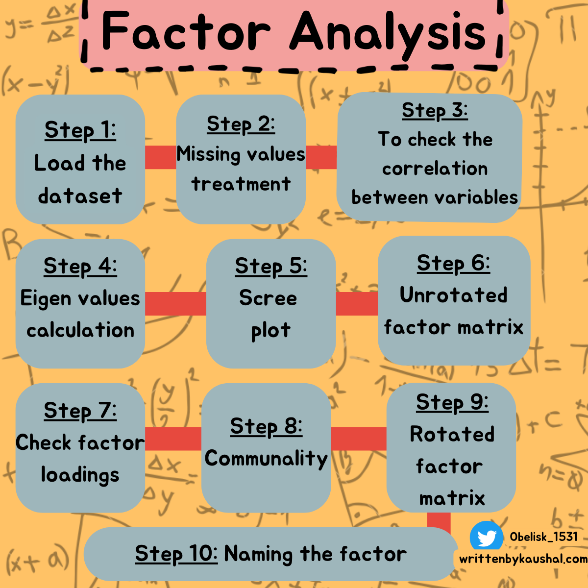
There are 10 steps in the application of Factor analysis.

Application of Factor analysis

So far you have learned what actually Factor analysis is. Let's look at the project that I have made in R language.

At the end of this story, I’ll share my repository link.

The dataset I used for this project is available on Kaggle. (here)

You can directly copy & edit my notebook. (link)

Step 1: Read and understand the dataset

hotel_data <- read.csv('../input/europe-hotel-satisfaction-score/Europe Hotel Booking Satisfaction Score.csv')
str(hotel_data)

Step 2: Checking missing value

install.packages("DataExplorer")
library(DataExplorer)

#missing value plot
plot_missing(hotel_data)

Step 3: Check the correlation between variables

Using cor() function we can find the correlation.

corrplot() will plot the correlation

Correlation can be performed onNumericdata only

# Correlation matrix
hotelcorr <- cor(hotel_data[, unlist(lapply(hotel_data, is.numeric))])

install.packages("corrplot")
library(corrplot)
corrplot(hotelcorr)

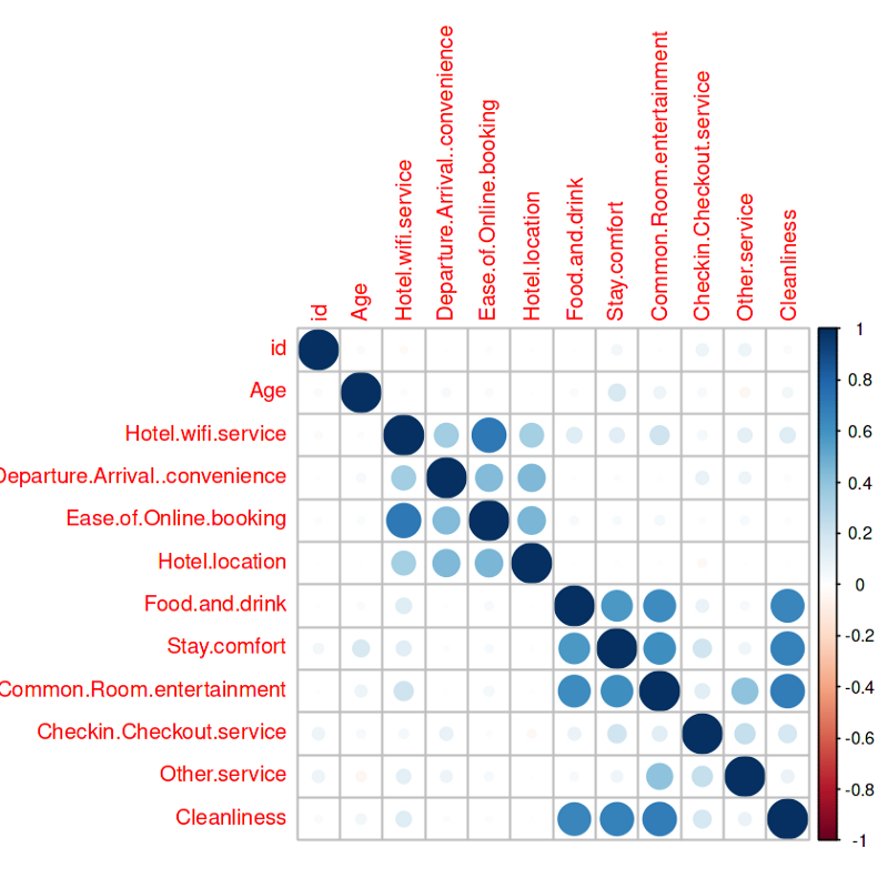
Note: Darker the color higher the correlation

The plot indicates a high correlation between the following variables-

• Hotel.wifi.service — Ease.of.Online.booking

• Cleanliness — Food.and.drink,Stay.comfort,Common.Room.entertainment

• Common.Room.entertainment — Food.and.drink, Stay.comfort

Step 4: Eigen value calculation

# Creating a variable hotel1, which is hotel_data - the dependent variable id
hotel1 <- (hotel_data[, unlist(lapply(hotel_data, is.numeric))])[-1]

#Eigen value
ev = eigen(cor(hotel1))
ev

Our dataset has 11 numeric variables, therefore 11 factors are created. The Eigenvalue indicates the variance & is always presented in decreasing order.

eigen() decomposition

$values

[1] 3.1195677 2.3229862 1.2092234 1.0255424 0.8545620 0.7607969 0.5381988

[8] 0.4012043 0.3035985 0.2584139 0.2059058

Here, the first four values have eigenvalues greater than 1, and therefore we have 4 factors.

Step 5: Scree plot

Scree plot helps in determining the optimal number of factors or components.

# Scree plot
install.packages("psych")
library(psych)

# Eigen values

EigenValues<- ev$values

# Listing of 11 factors
Factors=c(1,2,3,4,5,6,7,8,9,10,11)

#DataFrame with factors & Eigen values

Scree=data.frame(Factors, EigenValues)
plot(Scree, main="Scree Plot", col="black")
lines(Scree, col="red")

The eigenvalues & factors are plotted, and the point where the “elbow” shape is formed is considered.

In this plot 3 is the point where the elbow is formed. Therefore, the number of factors is considered as 3, which is the same result that the eigenvalues indicate.

Conclusion — from 11 variables, three factors can be derived.

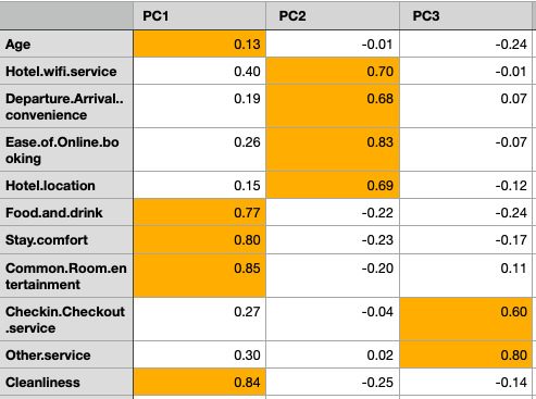
Step 6: Unrotated factor matrix

# Factor analysis - unrotated
# Here principal() function is used and rotation is kept as 'none'

hotel_unrotated = principal(hotel1, nfactors = 3, rotate='none')
hotel_unrotated

The unrotated factor matrix identifies factors based on the maximum variance. The output is a matrix showing the correlation between variables and the factor. PC1, PC2, and PC3 are the three principal components.

Step 7: Factor loadings

Based on the correlation the variables are loaded in factors as shown in the table. The variables with the highest correlation get loaded into the factor & which means the particular variable is representative of the factor.

The variable Age has a 0.13 correlation with PC1, which is highest among different components & therefore, gets loaded into PC1. Similarly other variables.

Step 8: Communality

• Communality is represented by h2 values, which show the variance of the variable captured by the component.

Hotel.wifi.service has h2 value of 0.650 which means 65% of the variance of the variable Hotel.wifi.service is captured in the components PC1 to PC3.

• The u2 values indicate the uniqueness of the variable(1-h2).

• SS-loadings indicate the sum of squared loadings, and a factor is considered good if the ss loading is greater than 1.

• The proportion variance of each component is explained in this part of the output. PC1 has 28%, PC2 has 21% & PC3 has 11%

• The cumulative variance gives the total of all four components, which is in this case 60%. This means 60% of the variance in the dataset is captured by the three components put together.

Step 9: Rotated factor matrix

• In order to get a more meaningful interpretation of the factors, the variables are rotated.

• In this notebook, we use varimax rotation, which is the most commonly used orthogonal rotation.

• As the name indicated, this method maximizes the variance between the factors.

• This drives all the lower correlations closer to zero & all the upper correlations closer to one.

# varimax rotation
hotel_rotate = principal(hotel1, nfactors = 3, rotate = 'varimax')
hotel_rotate
print("-----------------------------------")

#The factor loading is also represented as a diagram using the fa.diagram().

fa.diagram(hotel_rotate)

View(hotel1)
# combining the factors with the dataset
hotel_new <- cbind(hotel_data[1], hotel_rotate$scores)

Step 10: Naming the factors

# Labeling the data
names(hotel_new)<-c("Hospitality","Services & location","Value added services","Age")
head(hotel_new)

Make sure to go through the detailed code in my repository.

Here is the link to my GitHub repository(here).

Thank you for reading. For more such content make sure to subscribe to my Newsletter here
Make sure to Follow me on

Twitter

Linkedin

GitHub

Have a nice day 😁